Lecture 13
Optimization
APMA E2000
Drew Youngren dcy2@columbia.edu
Announcements
- Rec 7 this week
-
Quiz 3 this week (on Gradescope)
6pm Thurs–6pm Fri- Linearization
- Chain Rule
- Properties of $\nabla f$
- HW 7 due Tues
1-minute review
- Critical points of a function $f$ are those where $f$ is not differentiable or $\nabla f = 0$.
- Local mins and maxes (on open sets) only occur at critical points.
- The second derivative test can classify some critical points of $f(x,y)$.
Preliminaries
Kinds of Optimization
Unconstrained
On open sets $\longrightarrow$ look for critical points
Constrained
On boundary points $\longrightarrow$ Lagrange multipliers
Framework
For an optimization problem one must identify:
- The target function or desideratum $f$
-
The control variables $x, y, \ldots$
- Give description and units where appropriate
- The domain $D$ of admissible values
Example - Unconstrained
Find the closest point to the origin on the plane \[z = x - 2y + 3.\]
Solution. We will choose $x$ and $y$ freely (so $D = \RR^2$, open) and minimize the distance to $(x,y,x - 2y + 3)$. \[f(x,y) = x^2 + y^2 + (x - 2y + 3)^2\]
\[\nabla f = \bv{2x + 2(x - 2y + 3) \\ 2y - 4(x - 2y + 3)} = \bv{0 \\ 0}\] \[ = \bv{4x - 4y + 6 \\ - 4x + 10y - 12} = \bv{0 \\ 0}\]
\[ \implies y = 1, x = -\frac12 \]
which means the closest point is $(-1/2, 1, 1/2)$
Lagrange Multipliers
Constraint Function
In most real applications, we cannot choose out control variables freely, but rather they are subject to a constraint.
Often, we express this by specifying this as a level set \[g(x,y,\ldots) = k \]
e.g., a fixed budget or a set proportion of ingredients for a recipe.
What does the gradient tell us at local extremes on constrained sets?
Example
Identify the local minima of the distance to the Sun from a body restricted to the drawn "orbit".
Theorem - Lagrange Multipliers
A local minimum (or maximum) of $f(\vec x)$ subject to the constraint $g(\vec x) = k$ occurs at $\vec a$ only if $\nabla g(\vec a) = \vec 0$ or \[\nabla f(\vec a) = \lambda \nabla g(\vec a)\] for some scalar $\lambda$.
Example (Reprise)
Find the closest point to the origin on the plane \[z = x - 2y + 3.\]
Solution
Viewed as a constrained problem in $\mathbb{R}^3$, we target distance$^2$ and use the plane equation as the constraint. \[ f(x,y,z) = x^2 + y^2 + z^2,\ g(x,y,z) = x - 2y - z + 3 = 0 \]
\[ \nabla f = 2\bv{x \\ y \\ z} = \lambda \bv{1 \\ -2 \\ -1} = \lambda \nabla g\]
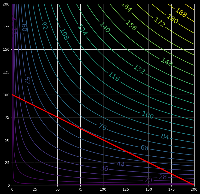
Example – Cobb-Douglass
By investing $x$ units of labor and $y$ units of capital, a low-end watch manufacturer can produce $x^{0.4}y^{0.6}$ watches. Find the maximum number of watches that can be produced with a budget of $\$20000$ if labor costs $\$100$ per unit and capital costs $\$200$ per unit.
Example – 3D
Find the minimum surface area of a lidless shoebox with volume $32 \text{ L}$.
XVT
Extreme Value Theorem
Theorem
A continuous function on a closed and bounded set $D$ must achieve its absolute minimum and maximum.
- Find critical points on interior of $D$.
- Find Lagrange points on boundary of $D$.
- Choose least/greatest value of $f$ on combined list.
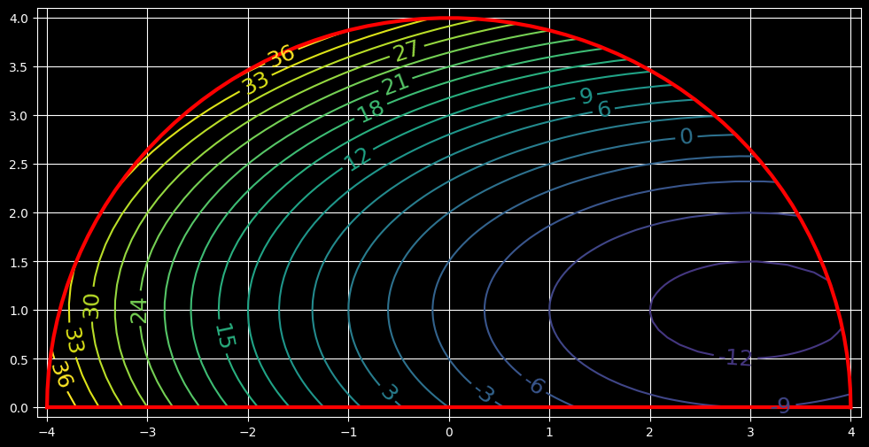
Example
Suppose the temperature distribution on the closed half-disk $0 \leq y \leq \sqrt{16-x^2}$ is given by \[u(x,y) = x^2 - 6x + 4y^2 - 8y. \] Find the hottest and coldest points.
Learning Outcomes
You should be able to...
-
Model an optimization problem by identifying:
- the target function.
- the variables and domain of feasibility.
- any constraint functions.
- Identify whether a domain is open, closed, or neither, and where to look for extrema.
- Set up and solve systems of equations for the method of Lagrange multipliers.
- Interpret the Lagrange equations geometrically.
- Utilize the Extreme Value Theorem to find global minima and maxima.