Lecture 16
Applications of Integration
APMA E2000
Drew Youngren dcy2@columbia.edu
Announcements
- HW 9 due next week.
-
Quiz 4 this week.
- Double/Triple Integrals
- Change of Coordinates
-
Exam 2 Tues, 03/31
- Same format as last time
- New seat assignments
- Not cumulative in the narrow sense but all math is cumulative.
1-minute review
Other Coordinates
- Polar coordinates $(r,\theta)$ \[ \iint_\mathcal R f(x,y)\,dxdy = \iint_\mathcal R f(r\cos \theta, r \sin \theta)\,r\,dr\,d\theta \]
Other Coordinates
- Cylindrical coordinates $(r,\theta, z)$\[ \iiint_\mathcal E f(x,y,z)\,dxdydz = \iiint_\mathcal E f(r\cos \theta, r \sin \theta,z)\,r\,dz\,dr\,d\theta \]
Other Coordinates
- Spherical coordinates $(\rho, \phi, \theta)$ \[ \iiint_\mathcal E f(x,y,z)\,dxdydz = \]\[\iiint_\mathcal E f(\rho \sin \phi \cos \theta, \rho \sin \phi \sin \theta, \rho \cos \phi ) \, \rho^2 \sin \phi \, d\rho \, d\phi \, d\theta \]
where the bounds of integration for $\mathcal R$ or $\mathcal E$ are translated appropriately.
Example
Find the volume of the "stadium" defined as the region above the $xy$-plane bound by a sphere of radius 2, a cylinder of radius 4, and the cone $x^2 + y^2 = z^2$, cut as shown.
\[ \int_{\pi/2}^{2\pi} \int_{\pi/4}^{\pi/2}\int_2^{4\csc \phi} \rho^2 \sin\phi \,d\rho\,d\phi\,d\theta = \]
\[ = (32 - 2\sqrt{2})\pi \]
Applied Integration
Applied Integration
The whole is the sum of its parts.
Density
Density, a rate of $\frac{\text{mass}}{\text{volume}}$ can vary continuously as a function of location $\mu(x,y,z)$. \[ \text{mass}_{\text{total}} = \iiint\limits_{\mathcal E} dm = \iiint\limits_{\mathcal E} \mu \,dV \]
but density can be more general: $\frac{\text{stuff}}{\text{space}}$.
Examples
- Resistivity $\mu(x)$ along a wire, $\frac{\Omega}{{\rm m}}$. \[\Omega = \int_0^\ell \mu(x)\, dx\]
- Probability density function $\mu(x,y)$ of two random variables. \[P(E) = \iint\limits_E \mu(x,y)\, dA\]
- Concentration of chemicals, like $[\text{H}_2\text{CO}_3] = \mu(x,y,z)$. \[\text{total carbonic acid} = \iiint\limits_D \mu(x,y,z)\,dV\]
Center of Mass
Discrete Mass Distribution
Suppose point masses $m_1$ and $m_2$ are located at positions $x_1$ and $x_2$, resp., along a line. The center of mass $\bar x$ is the position that balances the "moments".
\[m_1 (x_1 - \bar x) + m_2(x_2 - \bar x) = 0\]
Discrete Mass Distribution
Suppose point masses $m_1$ and $m_2$ are located at positions $x_1$ and $x_2$, resp., along a line. The center of mass $\bar x$ is the position that balances the "moments".
\[\bar x = \frac{m_1 x_1 + m_2 x_2}{m_1 + m_2}\]
Discrete Mass Distribution
Suppose point masses $m_1$ and $m_2$ are located at positions $x_1$ and $x_2$, resp., along a line. The center of mass $\bar x$ is the position that balances the "moments".
\[\bar x = \frac{m_1}{m_1 + m_2} x_1 + \frac{m_2}{m_1 + m_2} x_2\]
aka, a weighted average of the positions.
Continuous Mass Distribution
Suppose mass is distributed continuously along the interval $a \leq x \leq b$ with density $\mu(x)$. The center of mass $\bar x$ is the position that balances the "moments".
\[\int_a^b (x - \bar x) \mu(x)\,dx = 0\]
Continuous Mass Distribution
Suppose mass is distributed continuously along the interval $a \leq x \leq b$ with density $\mu(x)$. The center of mass $\bar x$ is the position that balances the "moments".
\[\bar x = \frac{\int_a^b x \mu(x)\,dx}{\int_a^b \mu(x)\,dx} \]
aka, a weighted average of the positions.
Higher Dimensions
A solid region $\mathcal E$ with continuously varying density (mass per unit volume) $\mu(x,y,z)$ has total mass \[M = \iiint_\mathcal E \mu(x,y,z)\,dV.\]
The center of mass $(\bar{x},\bar y,\bar z)$ is the (weighted) average position of the mass in the object. More concisely, \[\bv{\bar{x} \\ \bar{y} \\ \bar{z}} = \frac1M \bv{\iiint_\mathcal E x \mu(x,y, z)\,dV \\ \iiint_\mathcal E y \mu(x,y, z)\,dV \\ \iiint_\mathcal E z \mu(x,y, z)\,dV}\]
Example
The nose of a race car is modeled by half of a right cone with height $h$ and radius $R$. Assuming uniform density, how high is the center of mass from the bottom.
Solution.
Reorient
with cylindrical coords so that
$0 \leq \theta \leq \pi$, $0 \leq r \leq R$, $0 \leq z \leq h -
\frac{h}{R} r$
and $y$ is then the "height" coordinate.
\[ \bar{y} = \frac1V \iiint\limits_{\mathcal C} y\,dV \]
\[ = \frac{1}{\pi R^2 h / 6} \int_0^\pi \int_0^R \int_0^{h - \frac{h}{R}r} r^2 \sin\theta\,dz\,dr\,d\theta \] \[ = R / \pi \]
Moment of Inertia
Concept
CoM measures where mass is located on average. It can't measure how far it is spread out.
The moment of inertia does this. For a mass distribution $\mu(x,y,z)$ and a particular axis of rotation, \[ I = \iiint\limits_{\mathcal E} (\text{distance to axis})^2 \mu(x,y,z)\,dV \]
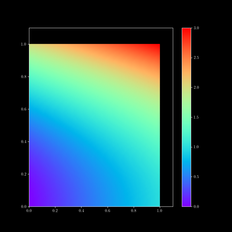
Example
Find the center of mass and the moments of inertia about the standard axes for a mass distribution $\mu$ on the unit square in $xy$.
\[\mu(x,y) = x + 2 y^2 \] in units of mass/area.
\[\bar{x} = \frac{\int_0^1\int_0^1 x (x + 2y^2)\,dy\,dx}{\int_0^1\int_0^1 (x + 2y^2)\,dy\,dx} = \frac47\]
\[\bar{y} = \frac{\int_0^1\int_0^1 y (x + 2y^2)\,dy\,dx}{\int_0^1\int_0^1 (x + 2y^2)\,dy\,dx} = \frac{9}{14}\]
\[I_{x} = \int_0^1\int_0^1 y^2 (x + 2y^2)\,dy\,dx = \frac{17}{30}\]
\[I_{y} = \int_0^1\int_0^1 x^2 (x + 2y^2)\,dy\,dx = \frac{17}{36}\]
MoI Examples
Find an expression for the moment of inertia $I$ (about a central axis) in terms of the total mass $M$ (with uniform density) for the following shapes:
- Cube with side $2R$.
- Right cone with base radius $R$ and height $h$.
- Half-ball with radius $R$.
Learning Outcomes
You should be able to...
- Interpret a density function (in various dimensions) as a distribution or an indication of "where stuff is."
- Correctly compute center of mass for various distributions, using symmetric arguments where appropriate.
- Reason about and compare moments for different distributions without necessarily computing the numeric value.
- Reinterpret basic probability questions about multiple random variables in terms of integrals.